Yesterday I had a chat with old Cetis friend Sheila, we got on to the conversation of visualising text, something I am really interested in but also really struggle with. Sheila had been playing with Textexture a tool to visualise any text as a network, I was intrigued by Sheila’s post and decided to do some experiments of my own trying different ways to visualise blog comments. Here are some of my own quick experiments and thoughts on them while I was playing with Textureture and trying to create something similar in R/Gephi.
Just a note that I’m not sure how useful any of these methods are yet. Its very much a ‘try it and see’ at this stage.
Grabbing the data
I’m using my own blog comments, I grabbed a CSV through a quick SQL query. You should have changed your prefix during installation, but the query might look something like this:
select * from wp_comments where `comment_approved` = 1
You could also use a wordpress plugin or good old copy paste. I have used all my comments since June 2013 which was when I started this blog (I have imported older blogs and since but not included the comments in this)
Textexture
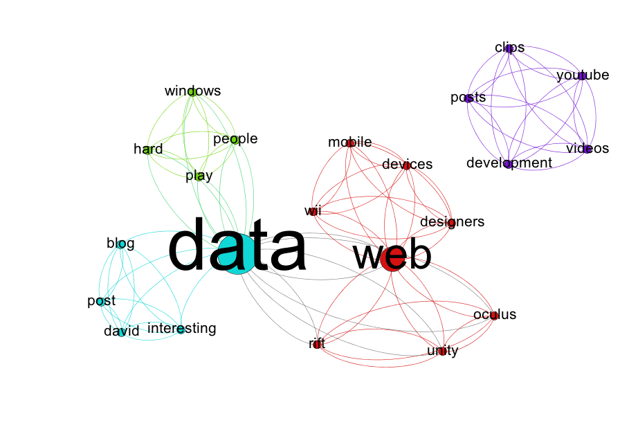
Sheila put me on to Textexture during our chat, it creates a network graph of your text similar to something you might see in Gephi. There is not much to describe of a recipe to describe in terms of how to use Textexture, it just requires you create a login and copy and paste your text in to the site. I took all my comments and copied them in and it returned something like this below graph. While I am all for pretty interactive pictures that are easy to do, it still leaves me wondering what it actually means. While it is hard to work out what we are looking at from the picture there is a methodology section on the textexture site. From a quick scan it appears that each node represents a word and a relationship between nodes is worked out through a bunch of things such as being next to each other in the text. Other things such as sentence structure are taken in to account, but some of the algorithms were beyond a quick scan. The size of the nodes relate to betweeness centrality and colour coding seems to be based on louvain modularity method. You can embed the interactive graph in to your site, it would have been nice if I could download the graph file to import in to Gephi itself but I’m not sure this really fits their business model. Here was the result from copy and pasting my comments:
Networks of Topic Models
I wanted to create something similar myself but felt that the sheer number of nodes in the thing created by Textexture made it a bit hard to suggest. I wrote a small script to generate abstract topics made up of keywords from my text and then wondered if I could create a network graph from them instead. I’m not sure how well this work, but I decided to build a network diagram with nodes representing words and edges meaning that the words share a topic.
The process wasn’t too hard, but a more work than copying and pasting in to textexture. First you need to generate some topic models using something like Mallet. If you wish to use the RMallet package Ben Marwick has excellent examples on his github. I generated 5 topics, each with 5 keywords that describe the comments. The comments can belong to multiple topics. The thing I took away from this exercise is that topic models don’t work on such small amount of texts, or at least they don’t work without lots of fine tweaking to the paramaters in mallet, for which I do not know enough. To generate topic models using Mallet I used a modified version of Ben’s script:
options(mc.cores=1)

documents <- data.frame(id = character(252),
                 text=character(252),
                 stringsAsFactors=FALSE)

comments<-read.csv("commentscsv.csv", sep = "," , header = TRUE)

comments = as.data.frame(sapply(comments, tolower))
comments = as.data.frame(sapply(comments, removeNumbers))
comments = as.data.frame(sapply(comments, stripWhitespace))
comments = as.data.frame(sapply(comments, skipWords))
commentdf<-data.frame(comments$comment_content)

documents$text  = comments$comment_content
documents$id <- Sys.time() + 30 * (seq_len(nrow(documents))-1)
documents <- data.frame(lapply(documents, as.character), stringsAsFactors=FALSE)

require(mallet)
mallet.instances <- mallet.import( documents$text ,  documents$text , "stoplists/en.txt", token.regexp = "\\p{L}[\\p{L}\\p{P}]+\\p{L}")

## Create a topic trainer object.
n.topics <- 20
topic.model <- MalletLDA(n.topics)

#loading the documents
topic.model$loadDocuments(mallet.instances)

## Get the vocabulary, and some statistics about word frequencies.
##  These may be useful in further curating the stopword list.
vocabulary <- topic.model$getVocabulary()
word.freqs <- mallet.word.freqs(topic.model)

## Optimize hyperparameters every 20 iterations,
##  after 50 burn-in iterations.
topic.model$setAlphaOptimization(20, 50)

## Now train a model. Note that hyperparameter optimization is on, by default.
##  We can specify the number of iterations. Here we'll use a large-ish round number.
topic.model$train(200)

## NEW: run through a few iterations where we pick the best topic for each token,
##  rather than sampling from the posterior distribution.
topic.model$maximize(10)

## Get the probability of topics in documents and the probability of words in topics.
## By default, these functions return raw word counts. Here we want probabilities,
##  so we normalize, and add "smoothing" so that nothing has exactly 0 probability.
doc.topics <- mallet.doc.topics(topic.model, smoothed=T, normalized=T)
topic.words <- mallet.topic.words(topic.model, smoothed=T, normalized=T)

# from http://www.cs.princeton.edu/~mimno/R/clustertrees.R
## transpose and normalize the doc topics
topic.docs <- t(doc.topics)
topic.docs <- topic.docs / rowSums(topic.docs)

## Get a vector containing short names for the topics
topics.labels <- rep("", n.topics)
for (topic in 1:n.topics) topics.labels[topic] <- paste(mallet.top.words(topic.model, topic.words[topic,], num.top.words=5)$words, collapse=" ")
# have a look at keywords for each topic
topicsforsubreddit<-topics.labels

# create data.frame with columns as authors and rows as topics
topic_docs <- data.frame(topic.docs)
names(topic_docs) <- documents$id

topics.labels
The 5 topics were:
post,david,interesting,blog,data
hard,play,people,data,windows
youtube,posts,videos,clips,development
oculus,web,rift,data,unity
mobile,web,devices,wii,designers
I turned each word in to a node with a relationship between nodes when sharing a topic and used Gephi’s modularity algorithm to find and colour communitys.
The Trusty Wordl
While in R it is quite easy to turn a word document matrix in to a word cloud, following on from the code above:
require("tm")

#corpus <- Corpus(DataframeSource(commentdf))
corpus <- Corpus(VectorSource(comments$comment_content)) # create corpus object
corpus.p <-tm_map(corpus, removeWords, stopwords("english")) #removes stopwords
corpus.p <-tm_map(corpus.p, stripWhitespace) #removes stopwords
corpus.p <-tm_map(corpus.p, removeNumbers)
corpus.p <-tm_map(corpus.p, removePunctuation)
dtm <-DocumentTermMatrix(corpus.p)

library("wordcloud")
word_frequency <- colSums(as.array(dtm))
wordcloud(names(word_frequency), word_frequency, scale=c(3,.5),
          max.words = 75, random.order=FALSE, colors=c("lightgray", "darkgreen", "darkblue"), rot.per=.3)
Output:
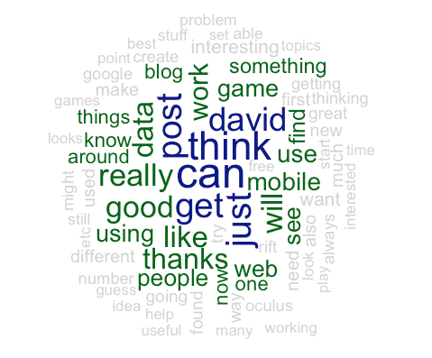
While Wordls get a bit of stick for being easy to do and consequently a bit overused I think they are a really good way to get across the themes that people are talking about. I wondered if we could spruce it up a bit and do a wordl of terms. I wrote a very quick loop to find ngrams from my comments:
for (i in 2:6 ) {
  nam <- paste( i, "grams", sep = "")

  #tokenizer for tdm with ngrams
  BigramTokenizer <- function(x) NGramTokenizer(x, Weka_control(min = i, max = i))
  tdm <- TermDocumentMatrix(corpus, control = list(tokenize = BigramTokenizer))

  #create dataframe and order by most used
  rollup <- rollup(tdm, 2, na.rm=TRUE, FUN = sum)
  mydata.df <- as.data.frame(inspect(rollup))
  colnames(mydata.df) <- c("count")
  mydata.df$ngram <- rownames(mydata.df)
  #newdata <- mydata.df[order(-count),]
  newdata<-mydata.df[order(mydata.df$count, decreasing=TRUE), ]
  assign(nam, newdata )
  filename<-paste(i,"gram",".csv")
  write.csv(newdata, file = filename)
}
I ‘wordled’ the phrases and wasn’t sure about the result”
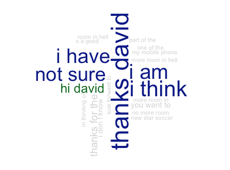
At this stage I think lots of the processes such as pulling out abstract topics, regular phrases etc are pretty useful but I’m not sure about the visualisation methods for them. Time for a sleep on it before I try again..
0 Comments