Testing creation of intensity maps from Wikipedia

I wanted to come up with a quick method that I could reuse where I could ask Wikipedia a quick question, get some numbers and create a heat map. I still haven’t come up with the quick process, and when I mess with data I tend to stick with what I know for a ‘first pass’ at the process and then cut down the steps when I know that it works. I guess other people who play with R packages will understand the frustration of spending 3 hours with a new R package only to learn that the process doesn’t work anyway and it would have been quicker just to have do the data mangling in Excel first before trying to create a repeatable process. These are the steps I went through to see if it was possible. I know that the data is incorrect, this seems to mainly be because of a problem with my SPARQL query.

1) Grab the data

I’m using DBpedia to get the data. I wanted to write query where I could just grab all the instances of something and then be able to put them on an intensity map. I picked any old question. I went with birthplace of all footballers that have played in the Premier League and using DBpedia this SPARQL query I came up with, this will get their town with its long and lat data:

SELECT ?person ?name ?born ?gps ?label WHERE {
?person dcterms:subject category:Premier_League_players.
?person rdfs:label ?name
FILTER ( lang(?name) = 'en' ) .
?person dbpedia-owl:birthPlace ?born .
?born rdf:type dbpedia-owl:City .
?born grs:point ?gps .
?born rdfs:label ?label
FILTER(LANG(?label) = '' || LANGMATCHES(LANG(?label), 'en'))

I used the SPARQL package in R to to do the query and write the results to CSV:

endpoint <- "http://live.dbpedia.org/sparql"
endpoint <- "http://dbpedia.org/sparql"
options <- NULL

query = "

PREFIX owl: <http://www.w3.org/2002/07/owl#>
PREFIX xsd: <http://www.w3.org/2001/XMLSchema#>
PREFIX rdfs: <http://www.w3.org/2000/01/rdf-schema#>
PREFIX rdf: <http://www.w3.org/1999/02/22-rdf-syntax-ns#>
PREFIX dc: <http://purl.org/dc/elements/1.1/>
PREFIX dbpedia: <http://dbpedia.org/>
PREFIX dcterms: <http://purl.org/dc/terms/>
PREFIX category: <http://dbpedia.org/resource/Category:>
PREFIX grs: <http://www.georss.org/georss/>

SELECT ?person ?name ?born ?gps ?label WHERE {
?person dcterms:subject category:Premier_League_players.
?person rdfs:label ?name
FILTER ( lang(?name) = 'en' ) .
?person dbpedia-owl:birthPlace ?born .
?born rdf:type dbpedia-owl:City .
?born grs:point ?gps .
?born rdfs:label ?label
FILTER(LANG(?label) = '' || LANGMATCHES(LANG(?label), 'en'))
}
"

qd <- SPARQL(endpoint,query)
df <- qd$results
write.csv(df, file = "footballersborn.csv")

I like to play with my data in OpenRefine before I do anything.. this isn’t a step that I would really need to do as I’m sure I could do some of my data cleansing in R, but for a first pass at things its just easier and quicker to have a look at the data and see what sort of stuff I need to clean up. In this case I just created two new columns, these were separate long and lat columns based from the GPS column.

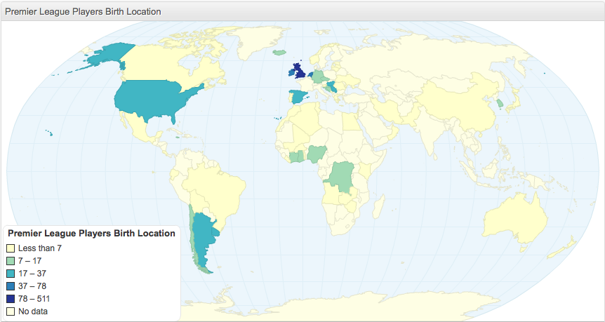
At this stage I noticed something fishey about my dataset, I’m guessing that there was either  something wrong with my query or the dataset, the biggest giveaway seemed to be that according to my dataset there were no footballers who have played in Premier League from France. I decided to press on anyway as this exercise was more about creating a repeatable process for now. At this stage it is very easy to plot the data as a punch of pins on Google Maps using Google Fusion Tables, I’ve done something similar before using the birth place of wrestlers. However, I wanted to create an intensity/choropleth map which is slightly different, Google Fusion Tables classic is supposed to do this, but the new version only creates heatmaps.

To have a go at doing this I needed to count up the number of occurrences of births of footballs from each country. I didn’t have country information in my dataset, so I quickly wrote a function to take the long and lat columns and create a dataframe of countriy codes. I then attached this dataframe to my old one, anybody who copies this will need to create an account at geonames.org and replace the username:

test <- function(test) {connectStr <- paste('http://ws.geonames.org/countryCode?lat=',test[7],'&lng=',test[6],'&username=user' , sep="")
                        con <- url(connectStr)
                        data<-readLines(con)
                        close(con)
                        return (data)}

ccodes<-apply(footlonglat, 1, test)
footlonglat$ccodes <- ccodes

I then counted the occurrences of county codes and wrote it to CSV.

number_of_players<-table(footlonglat$ccodes)
write.csv(number_of_players, file = "noplayers.csv")

The aim of this was to get it in to Google Fusion Tables and merge the table with a public table that had country codes and kmz details. This worked and the classic view was able to create an intensity map. The problem was while the process seemed to work, the map didn’t do anything. It could be because the data was small, or that Google Fusion Classic is on the way out, or that I just can’t use Google Fusion Tables properly… more experiments required.

I was able to load the CSV straight to chartsbin, which created this:

There is a choropleth package for R, which is the next thing to try to cut down the steps.